Quantum Algorithm Implementation: Finding the Best Deals

Introduction

The similarity between the rich and the poor is that both love a good bargain - just at different stores. Whether you’re shopping at Louis Vuitton or a local flea market, everyone is on the lookout for the best deals. But what if you could use cutting-edge technology to optimize your shopping experience? Imagine trying to bundle purchases to maximize discounts, but the options are so numerous, forget about manually evaluating each one, it’s impossible even for today’s supercomputers. However, this problem can be tackled using quantum computing, specifically with the BILP-Q algorithm. Let’s dive into how this works.

Understanding the Basics

What is the Problem?

Think of this as a shopping challenge. You have four items to buy: a webcam, shoes, headphones, and socks. Each item or combination of items has a different discount. The goal? Find the best combination of bundles to minimize your total cost.

Classical Approach vs. Quantum Approach:

Traditionally, solving this involves evaluating all possible combinations of items, which quickly becomes impractical as the number of items increases. This is a well-known NP-Hard problem in AI called the Coalition Structure Generation (CSG) problem which has vital applications in cooperative game theory, multi-agent systems, and microeconomics. Quantum computing, however, can handle this complexity more efficiently.

Introducing BILP-Q

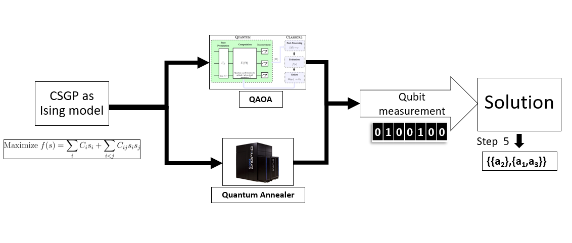
BILP-Q stands for Binary Integer Linear Programming - Quantum. It transforms our shopping problem into a Quadratic Unconstrained Binary Optimization (QUBO) problem, which quantum computers can solve effectively using algorithms like Quantum Approximate Optimization Algorithm (QAOA).

Example Scenario

Imagine you want to buy four items: a webcam, shoes, headphones, and socks. Here’s how the discounts for different bundles look:

Single items:

• Webcam: $30
• Shoes: $40
• Headphones: $25
• Socks: $15

Bundles of two items:

• Webcam & Shoes: $50
• Webcam & Headphones: $40
• Webcam & Socks: $50
• Shoes & Headphones: $55
• Shoes & Socks: $45
• Headphones & Socks: $45

Bundles of three items:

• Webcam, Shoes & Headphones: $90
• Webcam, Shoes & Socks: $95
• Webcam, Headphones & Socks: $75
• Shoes, Headphones & Socks: $85

All four items:

• Webcam, Shoes, Headphones & Socks: $105

Your goal is to buy all four items with the maximum discount, or in other words, with the least total cost.

For formal definitions of the problem and mathematical details, please refer to the original paper of BILP-Q.

Visual Representation of the solution space

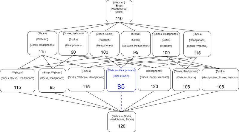
The following diagram shows all possible ways to purchase the four items, along with their total costs.

Each level represents a different number of groups (coalitions). The blue-colored cell denotes the best option to buy as it has the least cost. In this example, the optimal way to purchase all items is by splitting them into two groups: {Shoes, Socks} and {Webcam, Headphones}, with a total cost of $85Manually checking each possible combination is tedious, so we use BILP-Q to find the optimal solution.

Walkthrough of BILP-Q solution

Setting Up the Problem:

Installation

Clone the Repository:

Begin by cloning the BILP-Q repository to your local machine. Open a terminal/cmd/powershell and run

git clone https://github.com/supreethmv/BILP-Q.git
cd BILP-Q

Set Up a Virtual Environment (Optional):

Following good practices and to avoid dependency conflicts, create and activate a virtual environment.

python3 -m venv bilpq_env # or `virtualenv bilpq_env`
source bilpq_env/bin/activate  # On Windows, use `bilpq_env\Scripts\activate`

Install Dependencies:

Use the provided requirements.txt to install all necessary libraries. The process may take a few minutes depending on your internet speed and the packages already available in your system.

pip install -r requirements.txt

Install qiskit:

jupyter notebook notebook.ipynb

This command will create a new notebook with the specified name notebook.ipynb and open it in your web browser.

Run the below python code one-by-one in the opened jupyter notebook

import Utils_Solvers
import Utils_CSG

Define the Problem Instance:

We will enumerate the items as follows: 

1. for Webcam,
2. for Shoes, 
3. for Headphones, and 
4. for Socks.

Here’s how you can initialize the problem instance as a python dictionary:

# Define the cost of each bundle
coalition_values = {
 "1": 30,
 "2": 40,
 "3": 25,
 "4": 15,
 "1,2": 50,
 "1,3": 40,
 "1,4": 50,
 "2,3": 55,
 "2,4": 45,
 "3,4": 45,
 "1,2,3": 90,
 "1,2,4": 95,
 "1,3,4": 75,
 "2,3,4": 85,
 "1,2,3,4": 105
}

Convert to BILP:

We convert the CSG problem to a Binary Integer Linear Programming (BILP) problem:

c, S, b = Utils_CSG.convert_to_BILP(coalition_values)

Convert to QUBO:

Next, we convert the BILP problem to a Quadratic Unconstrained Binary Optimization (QUBO) problem:

import numpy as np
qubo_penalty = 50 * -1
linear, quadratic = Utils_CSG.get_QUBO_coeffs(c, S, b, qubo_penalty)
Q = np.zeros([len(linear), len(linear)])
for key, value in linear.items():
  Q[int(key.split('_')[1]), int(key.split('_')[1])] = value
# Non-diagonal elements
for key, value in quadratic.items():
  Q[int(key[0].split('_')[1]), int(key[1].split('_')[1])] = value / 2
  Q[int(key[1].split('_')[1]), int(key[0].split('_')[1])] = value / 2

Solving QUBO Using QAOA:

We use QAOA to solve the QUBO problem:

backend = BasicAer.get_backend('qasm_simulator') 
optimizer = COBYLA(maxiter=100, rhobeg=2, tol=1.5)
qubo = create_QUBO(linear, quadratic)
p=1
init = [0.,0.]
qaoa_mes = QAOA(optimizer=optimizer, reps=p, quantum_instance=backend, initial_point=init)
qaoa = MinimumEigenOptimizer(qaoa_mes) # using QAOA
qaoa_result = qaoa.solve(qubo)
solution = qaoa_result.x
print(f'Solution: {solution}')

Decoding the Solution:

The solution is a binary string of size 2^n-1, where each bit represents a non-empty subset of the items, and the positions marked 1 will be considered.

In our example, for four items, the subsets are:

1. Webcam
2. Shoes
3. Headphones
4. Socks
5. Webcam, Shoes
6. Webcam, Headphones
7. Webcam, Socks
8. Shoes, Headphones
9. Shoes, Socks
10. Headphones, Socks
11. Webcam, Shoes, Headphones
12. Webcam, Shoes, Socks
13. Webcam, Headphones, Socks
14. Shoes, Headphones, Socks
15. Webcam, Shoes, Headphones, Socks

The basis states of the qubits in the quantum circuit that solve the QUBO problem are measured, and there are only two basis states of a qubit |0⟩ or |1⟩ which can be interpreted as binary. Hence, the solution is obtained as a binary string.
For the shopping example, the solution obtained will look like 000001001000000.

Parsing the binary string from left to right, we select the 6th subset 1,3⇒Webcam, Headphones and the 9th subset 2,4⇒Shoes, Socks as the optimal bundles to purchase.

So, the solution to this problem is the set of mutually exclusive subsets of the items, such that each item occurs in exactly one of the subsets, i.e., {{Webcam, Headphones}, {Shoes, Socks}}.

Visualizing the Quantum Circuit:

You can also display the quantum circuit used in QAOA:

qaoa_mes.get_optimal_circuit().draw('mpl') 

You can also run this on a real hardware by signing-up to IBM’s Quantum Lab.

The Challenge of the Problem

Although this is a very hard problem, the size of the input is also exponential compared to the number of agents (items in this case). For n=4 items, the input was a dictionary of prices for each possible bundle, which totals 2^n−1 = 2⁴−1=15. Since every possible bundle is measured as a basis state of a unique qubit, the number of qubits scale exponentially with the number of items.

Thus, in the next post, we will explore induced subgraph games, where the problem setting is more practical, but the complexity of finding the optimal solution is still hard for classical computers.

Conclusion

In this post, we explored how a quantum algorithm can tackle complex optimization problems efficiently. We have modeled a very primitive scenario while the actual problem is based on intelligent agents and typically not items. There are more realistic coalition formation use cases that can be implemented such as peer-to-peer energy trading, logistics, wireless sensor networks, portfolio optimization, and see how quantum computing can simplify the decision-making process.

Quantum computing is still emerging, but its potential to solve complex optimization problems is immense. As quantum technology advances, we can expect more efficient solutions to problems that are currently infeasible for classical computers.

References

• Supreeth Mysore Venkatesh, Antonio Macaluso, and Matthias Klusch. “BILP-Q: Quantum Coalition Structure Generation.” 19th ACM International Conference on Computing Frontiers (CF’22), May 17–19, 2022, Torino, Italy. Paper Link, arXiv Preprint

• Github repository: https://github.com/supreethmv/BILP-Q

You can get more mathematically detailed explanation of an example in the tutorial notebook: https://github.com/supreethmv/BILP-Q/blob/main/BILP_Q_Tutorial.ipynb